| |
Seafloor mapping is largely a matter of measuring depth. Prior to the First World War, the depth of the oceans was usually measured by lead lining. This involved lowering a chunk of lead (usually a cannonball) on a very long piano wire to the bottom of the sea. In 1826, Daniel Colladon measured the speed of sound in the waters of Lake Geneva, Switzerland. This experiment was one of many steps toward the creation of sonar. However, using sonar remained in the experimental stage for another 90 years, and sailors continued to make their measurements the old fashioned way.
The First World War changed all this when Germany put submarines into action against Allied ships. The ships had no way of seeing the submarines coming. The U.S. War Department asked scientists what could be done about this problem. The resulting war effort produced (a) government funding of research and (b) anti-submarine warfare, which resulted in the accelerated development of underwater technology. Submarines also benefited from echo technology when sound sources were installed on the submarines for both echolocation and Morse code.
After using underwater sound technology for measuring the proximity to the shore and other ships, researchers soon realized that if the sound device was pointed down at the seafloor, the depth could be accurately determined. Early "echo sounders", as they were called, had very poor directivity, and relied on the assumption that the echoes were coming from directly beneath you. The included angle (cone of the beam pattern out to the 3 dB down point) was about 60 degrees. This was a poor assumption if there was any shape to the seafloor below (see figure below) but was easier than the old lead line method, and could be carried out while under way.
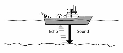
Figure 1 shows a typical echo sounder’s dynamics
Marine Geology, which was a relatively new science at the time, also helped with the development of sonar.
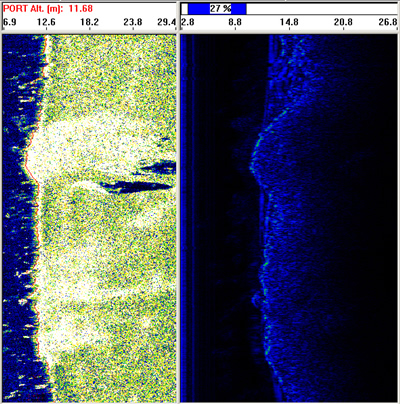
Figure 2 shows a comparison of bottom tracking and subbottom profile, from SIS-1000 data
Marine Geologists found that if you put enough energy into the "ping" you could get echoes from the layers of sediments and rocks beneath the bottom profile, and called this the "sub-bottom profile" (Figure 2). By recording the amplitude of the backscatter energy as a function of time and making some assumptions about sound velocity in the water (1500 m/sec) and the rocks (faster than 1500 m/sec), marine geologists could convert this data into water depth and rock layer thickness. By pinging continuously, driving the boat in straight lines, and laying all the ping records next to each other, they got an image, which looked like a vertical profile through the water column and sub-bottom. Dark reflectors correspond to scattered energy from point scatterers or layer transitions, termed changes in acoustic impedance (density * compressional wave sound velocity in the upper layer divided by the same for the lower layer).
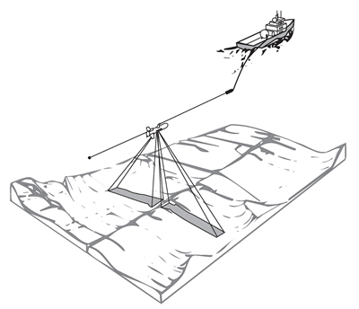
Figure 3 shows the geometry of a typical sidescan sonar.
Commercial aspects of sonar were quickly applied to the research (and drove it in many cases). Today, oil companies and geological surveyors record the echo profiles from towed hydrophone arrays in search of petroleum in the Gulf of Mexico and elsewhere with seismic sources (air guns, water guns, sparkers, explosives or other means); a method called seismic profiling. On the less costly and dangerous end, most research boats these days are equipped with 3.5Khz sub-bottom profilers which have a fairly wide beam (12-30 degrees) but good penetration (usually measured in fractions of a second, since we don't know the velocity of what we're penetrating). Alternatively, if better bathymetric profiles are required a higher frequency depth precision depth recorder, also known as a narrow beam sounder is required (at the expense of less penetration). These often operate at 12 KHz or above and have a single beam 2-4 degrees wide. With a narrower beam, you may have greater confidence that the value you pick as the bottom (from the first echo return) is actually right beneath you, and not off to the side (side-swipe).
While being able to continuously gather bathymetric profiles was a great improvement from the archaic lead lining method, it still meant you only knew what was right beneath you. Anything off to the side was still an unknown. Naturally, the next approach was to point the beams of the sonar out to the side, creating fan shaped beams to port (left) and starboard (right) which mapped a broad bow-tie shaped piece of the seafloor with every ping.
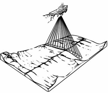
Figure 4 shows the geometry of a typical multibeam sonar for mapping ocean bottom contours.
MULTIBEAM
There are two main types of sonars; multibeam sonars for mapping bathymetry, and sidescan sonars for mapping seafloor imagery. Multibeam bathymetric mapping systems are straightforward in that they consist of a source transducer designed to ensonify a broad region out to either side (say 60 degrees out to either side, but only one or two degrees along the ship's track). They also involve a receiver array (hydrophones) that, through the magic of phase delay techniques, manages to pre-form multiple adjacent beams focused at known angles. As each 'beam' listens for returns from only one angle, but every beam records the time of the returning echoes independently, each ping results in "n" pairs of range (travel time * speed of sound / 2) and angle, where n is the number of beams. Range and angle for each beam can be converted to cross-track distance and depth. String all the points together, and you have a bathymetric surface you can contour or play with in many other fashions. More recently, people have begun to realize that you could not only log the time of the echo in each beam, but the amplitude as well, in order to determine how reflective the bottom was, as well as its depth/shape.
Some of the better-known multi-beam systems out there today are Odom, Reson 8101, & 9001, Sea Beam, Hydro sweep, Simrad-EM1000 and the Japanese MBES (multi-beam echo sounder). For reasons of convenience, multibeam systems are traditionally mounted on the hull of the vessel, and hence do better on calm days. While they are stabilized for ship motion, when the boat bangs around a lot, it tends to put both bubbles and noise in the water, which doesn't help the multibeam system. OIC works with data from all of these systems, and we have developed our own set of routines for processing both bathymetry and backscatter to minimize noise and other spurious data.
SIDESCAN
The second main type of marine survey device is a sidescan sonar, which, as the name implies, scan out to the side (this stuff isn't that hard is it?), illuminating a bowtie shaped area of the seafloor with each ping. Within this group, there are two sub-groups: sidescan-only systems, which only produce acoustic images of the seafloor; and bathymetric sidescan sonars, which create both bathymetry and sidescan. At OIC, we work with both sidescan and Multibeam sonars.
Sidescan sonars produce images of the seafloor and the objects on it. They do this by continuously pinging and recording backscattered echoes as a function of time, and stacking the echo traces to make images. Strong reflectors are traditionally plotted as dark, and shadows as light. If the raw echo time series is plotted with time increasing on the x-axis and ping number increasing on the y-axis, we have what we call raw, uncorrected or "slant-range" imagery.
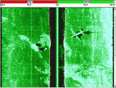
Figure 5 shows a sidescan image with the center track and data from the port and starboard channels.
Since the x-axis is travel-time, and the y-axis is distance along track (or ping number), you really can't use these slant-range images for accurate location or measurement of objects. However, if the height off the bottom (towfish altitude) is less than one quarter of the maximum slant range, they present reasonably undistorted images with minimal computational effort. Furthermore, they provide a clear indication of the bottom profile beneath the fish, which is quite useful in keeping the fish out of the mud (if the two sides were to close in and merge together, your water column would be zero, and you'd then be dredging, not surveying). While the echoes from objects in sidescan sonar images are sometimes fuzzy, the shadows are often quite crisp, as shown below.
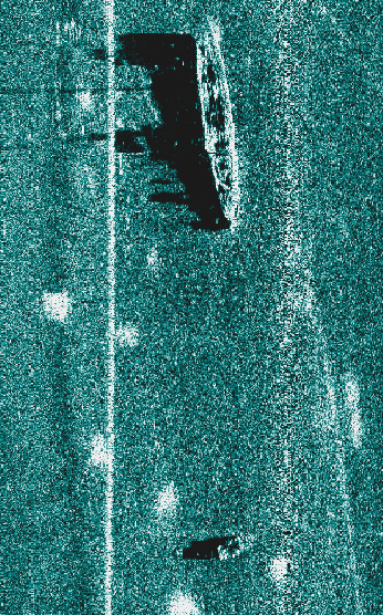
This sidescan image shows two submerged craft taken by the SIS1000
Another factor influencing images is the sonar frequency. As the speed of sound in water is relatively constant, at higher frequencies, the sound wavelengths are shorter. As sonar echo strength is proportional to target roughness at the wavelength of the sonar source, higher frequencies pick out finer roughness better, as seen in the images above.
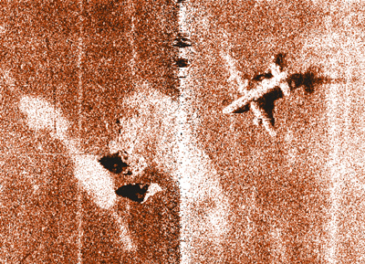
Man-made objects show up well in sidescan sonar images, as they usually have high acoustic impedance, and nice crisp sharp edges and corners as reflectors. However, as the image below shows, it's shape, not the intensity, that separates this plane from the surrounding rocks.
|